Design

This guide covers the library internals for contributors.

Module Architecture

Problem Model

Every problem implements Problem. The associated Value type is the per-configuration aggregate returned by evaluate(). Solvers fold these values across the configuration space, and witness-capable aggregates can also recover representative configurations.

trait Problem: Clone {
    const NAME: &'static str;              // e.g., "MaximumIndependentSet"
    type Value: Clone;                     // e.g., Max<i32>, Or, Sum<i32>
    fn dims(&self) -> Vec<usize>;          // config space per variable
    fn evaluate(&self, config: &[usize]) -> Self::Value;
    fn variant() -> Vec<(&'static str, &'static str)>; // e.g., [("graph", "SimpleGraph"), ("weight", "i32")]
    fn num_variables(&self) -> usize;      // default: dims().len()
    fn problem_type() -> ProblemType;      // default: registry lookup by NAME
}

• Problem — the base trait. Every problem declares a NAME (e.g., "MaximumIndependentSet"). The solver explores the configuration space defined by dims() and scores each configuration with evaluate(). For example, a 4-vertex MIS has dims() = [2, 2, 2, 2] (each vertex is selected or not); evaluate(&[1, 0, 1, 0]) returns Max(Some(2)) if vertices 0 and 2 form an independent set, or Max(None) if they share an edge. Each problem also provides inherent getter methods (e.g., num_vertices(), num_edges()) used by reduction overhead expressions.
• Witness-capable objective problems — typically use Max<V>, Min<V>, or Extremum<V> as Value.
• Witness-capable feasibility problems — typically use Or.
• Aggregate-only problems — use fold values such as Sum<W> or And; these solve to a value but do not admit representative witness configurations.
• Common aggregate wrappers — Max<V>, Min<V>, Sum<W>, Or, And, Extremum<V>, ExtremumSense.

Variant System

A single problem name like MaximumIndependentSet can have multiple variants — carrying weights on vertices, or defined on a restricted topology (e.g., king's subgraph). Variants form a subtype hierarchy: independent sets on king's subgraphs are a subset of independent sets on unit-disk graphs. The reduction from a more specific variant to a less specific one is a variant cast — an identity mapping where indices are preserved.

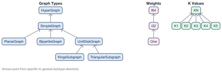
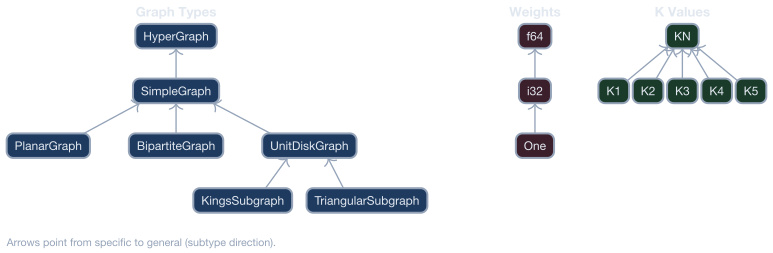
Variant types fall into three categories:

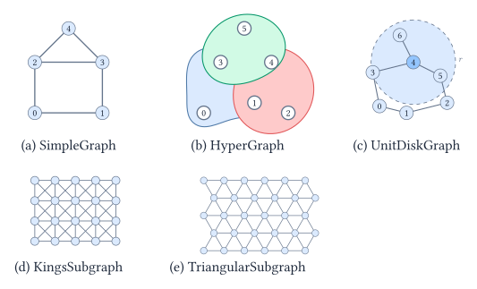
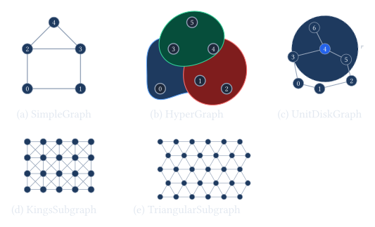
• Graph type — SimpleGraph (root), PlanarGraph, BipartiteGraph, UnitDiskGraph, KingsSubgraph, TriangularSubgraph.
• Weight type — One (unweighted), i32, f64.
• K value — e.g., K3 for 3-SAT, KN for arbitrary K.

pub trait VariantParam: 'static {
    const CATEGORY: &'static str;     // e.g., "graph", "weight", "k"
    const VALUE: &'static str;        // e.g., "SimpleGraph", "i32"
    const PARENT_VALUE: Option<&'static str>;  // None for root types
}

pub trait CastToParent: VariantParam {
    type Parent: VariantParam;
    fn cast_to_parent(&self) -> Self::Parent;
}

// Root type (no parent):
impl_variant_param!(SimpleGraph, "graph");

// K root (arbitrary K):
impl_variant_param!(KN, "k", k: None);

// Specific K with parent:
impl_variant_param!(K3, "k", parent: KN, cast: |_| KN, k: Some(3));

impl_variant_reduction!(
    MaximumIndependentSet,
    <KingsSubgraph, i32> => <UnitDiskGraph, i32>,
    fields: [num_vertices, num_edges],
    |src| MaximumIndependentSet::new(
        src.graph().cast_to_parent(), src.weights().to_vec())
);

// MaximumIndependentSet<G: VariantParam, W: VariantParam>
fn variant() -> Vec<(&'static str, &'static str)> {
    crate::variant_params![G, W]
    // e.g., MaximumIndependentSet<UnitDiskGraph, One>
    //     -> vec![("graph", "UnitDiskGraph"), ("weight", "One")]
}

Reduction Rules

A reduction requires two pieces: a result struct and a ReduceTo<T> impl.

The result struct holds the target problem and the logic to map solutions back:

#[derive(Debug, Clone)]
pub struct ReductionISToVC<W> {
    target: MinimumVertexCover<SimpleGraph, W>,
}

impl<W: WeightElement + VariantParam> ReductionResult for ReductionISToVC<W> {
    type Source = MaximumIndependentSet<SimpleGraph, W>;
    type Target = MinimumVertexCover<SimpleGraph, W>;

    fn target_problem(&self) -> &Self::Target { &self.target }
    fn extract_solution(&self, target_sol: &[usize]) -> Vec<usize> {
        target_sol.iter().map(|&x| 1 - x).collect()  // complement
    }
}

The #[reduction] attribute on the ReduceTo<T> impl registers the reduction in the global registry (via inventory):

#[reduction(overhead = {
    num_vertices = "num_vertices",
    num_edges = "num_edges",
})]
impl ReduceTo<MinimumVertexCover<SimpleGraph, i32>>
    for MaximumIndependentSet<SimpleGraph, i32>
{
    type Result = ReductionISToVC<i32>;
    fn reduce_to(&self) -> Self::Result { /* ... */ }
}

inventory::submit! {
    ReductionEntry {
        source_name: "MaximumIndependentSet",
        target_name: "MinimumVertexCover",
        source_variant_fn: || <MaximumIndependentSet<SimpleGraph, i32> as Problem>::variant(),
        target_variant_fn: || <MinimumVertexCover<SimpleGraph, i32> as Problem>::variant(),
        overhead_fn: || ReductionOverhead {
            output_size: vec![
                ("num_vertices", Expr::Var("num_vertices")),
                ("num_edges", Expr::Var("num_edges")),
            ],
        },
        module_path: module_path!(),
        reduce_fn: |src: &dyn Any| -> Box<dyn DynReductionResult> {
            let src = src.downcast_ref::<MaximumIndependentSet<SimpleGraph, i32>>().unwrap();
            Box::new(ReduceTo::<MinimumVertexCover<SimpleGraph, i32>>::reduce_to(src))
        },
    }
}

Reduction Graph

ReductionGraph::new() iterates all registered ReductionEntry items (via inventory) and builds a variant-level directed graph:

• Nodes are unique (problem_name, variant) pairs — e.g., ("MaximumIndependentSet", {graph: "KingsSubgraph", weight: "i32"}).
• Edges come exclusively from #[reduction] registrations — both cross-problem reductions and variant casts. There are no auto-generated edges.

Exported files:

• reduction_graph.json — all problem variants and reduction edges
• problem_schemas.json — field definitions for each problem type

These JSON assets are generated during make doc, make mdbook, and make paper; they are build artifacts, not committed source files. Generate them manually with cargo run --example export_graph and cargo run --example export_schemas when you need the raw exports locally.

Path finding

All path-finding operates on exact variant nodes. Use ReductionGraph::variant_to_map(&T::variant()) to convert a Problem::variant() into the required BTreeMap<String, String>.

Use find_cheapest_path with MinimizeSteps for fewest-hops search.

The PathCostFn trait (used by find_cheapest_path) computes edge cost from overhead and current problem size:

CustomCost wraps a closure that receives the edge's ReductionOverhead (polynomial mapping from input to output size fields) and the current ProblemSize (accumulated field values at that point in the path), and returns an f64 edge cost. Dijkstra minimizes the total cost along the path.

Example: Finding a path from MIS{KingsSubgraph, i32} to VC{SimpleGraph, i32}:

MIS{KingsSubgraph,i32} -> MIS{UnitDiskGraph,i32} -> MIS{SimpleGraph,i32} -> VC{SimpleGraph,i32}
     variant cast              variant cast                reduction

Executable paths

Convert a ReductionPath into a typed ExecutablePath<S, T> via make_executable(), then call reduce():

// find_cheapest_path returns a ReductionPath (list of variant node IDs)
let rpath = graph.find_cheapest_path("Factoring", &src_var,
    "SpinGlass", &dst_var, &ProblemSize::new(vec![]), &MinimizeSteps).unwrap();

// make_executable converts it into a typed, callable chain
let path = graph.make_executable::<Factoring, SpinGlass<SimpleGraph, f64>>(&rpath).unwrap();

// reduce() applies each step, returning a ChainedReduction
let reduction = path.reduce(&factoring_instance);
let target: &SpinGlass<SimpleGraph, f64> = reduction.target_problem();
let solution: Vec<usize> = reduction.extract_solution(&target_solution);

ExecutablePath holds a type-erased ReduceFn per edge. reduce() applies them sequentially, producing a ChainedReduction that stores each intermediate result. extract_solution maps the final solution back through the chain in reverse order.

For full type control, you can also chain ReduceTo::reduce_to() calls manually at each step.

#[reduction(overhead = {
    num_vars = "num_vertices + num_edges",
    num_clauses = "3 * num_edges",
})]
impl ReduceTo<Target> for Source { ... }

Input:  ProblemSize { num_vertices: 10, num_edges: 15 }
Output: ProblemSize { num_vars: 25, num_clauses: 45 }

Solvers

Solvers implement the Solver trait:

pub trait Solver {
    fn solve<P>(&self, problem: &P) -> P::Value
    where
        P: Problem,
        P::Value: Aggregate;
}

JSON Serialization

All problem types support JSON serialization via serde:

use problemreductions::io::{to_json, from_json};

let json: String = to_json(&problem)?;
let restored: MaximumIndependentSet<SimpleGraph, i32> = from_json(&json)?;

Contributing

See Call for Contributions for the recommended issue-based workflow (no coding required).